What is Convolutional Neuron Network?

Convolutional Neural Networks (CNNs) are also known as convnets. These types of deep learning models are widely used in computer vision applications.

In mathematics convolution is an operation on two functions to produce a third function that expresses how the shape of one is modified by the other.

In image processing convolution involves a kernel (small matrix) that is used for operations like blurring, sharpening, edge detection, etc. (Details about convolution in Image Processing)

Densely Connected Layer vs. Concolution Layer

Dense layers learn global patterns in their inputs. For example, densely connected deep learning model trained on the handwritten digit dataset learns patterns on 28 x 28 pixels. This can result it prediction errors for similar inputs, as shown below image.

By contrast, from the below image, we can see convolution layers learn local patterns found in small windows (the dimension of convolution kernel). For the handwritten digits dataset, using this technique results in prediction accuracy above 99%.

How does CNN Works?

The convolution operation

The patterns learned by CNNs are translation invariant. After learning a certain pattern in one part of an input image, a convnet can recognize it anywhere. This makes convnets data efficient when processing images.

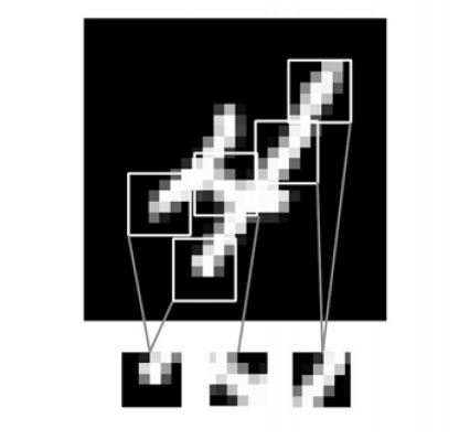
CNNs can learn spatial hierarchies of patterns. A first convolution layer will learn small local patterns such as edges, a second convolution layer will learn larger patterns made of the features of the first layers, and so on. This allows convnets to efficiently learn increasingly complex and abstract visual concepts. The below Image details how this process works

The visual world forms a spatial hierarchy of visual modules:
hyperlocal edges combine into local objects such as eyes or ears,
which combine into high-level concepts such as “cat.”

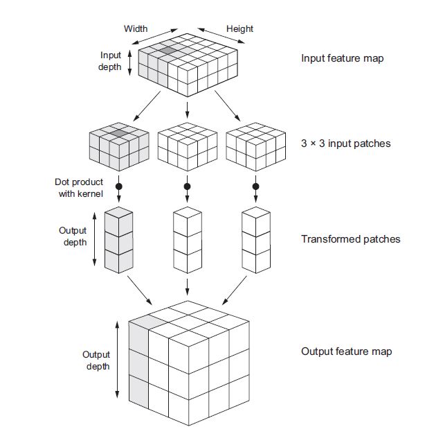
Convolutions operate on 3D tensor, called feature maps, with two spatial axis (height and width) as well as a depth axis(also called channels axis). For an RGB image, the dimension of the depth axis is 3, because the image has three color channels: red, green, and blue. For a black-and-white picture, like the MNIST digits, the depth is 1 (levels of gray).

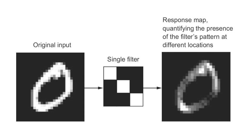
Then the convolution operation extracts patches from its input feature map and applies the same transformation to all of these patches, producing an output feature map (aka response map).

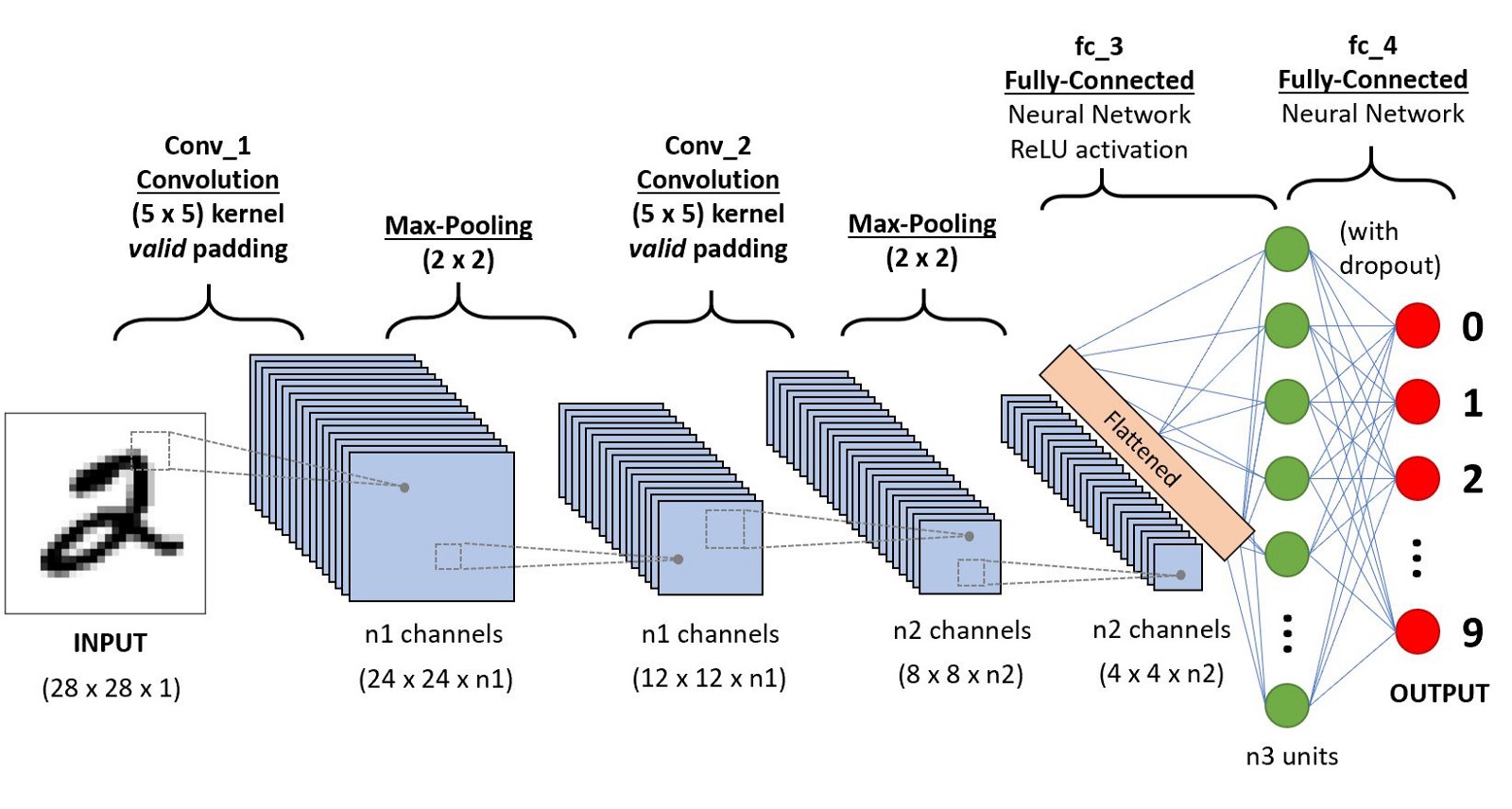
In the MNIST example, the first convolution layer takes a feature map of size (28, 28, 1) and outputs a feature map of size (26, 26, 32). It computes 32 filters over its input. Each of these 32 output channels contains a 26 × 26 grid of values, which is a response map of the filter over the input, indicating the response of that filter pattern at different locations in the input. (shown as below image)

Convolution works by sliding windows of size 3 × 3 on the 3D input feature map, extracting 3D patches. Each such 3D patch is then transformed into a 1D vector of shape. All of these vectors are then spatially reassembled into a 3D output feature map.(shown as below image)

Note that the output width and height may differ from the input width and height. They may differ for two reasons:

1. Border effects, which can be countered by padding the input feature map
2. The use of strides, which I’ll represents how many steps for each filtering.

The Border Effects and Padding in Convolution Operation

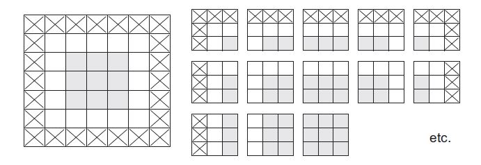
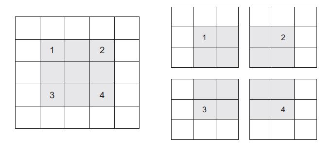
One factor that can influence output size is Border effects. Convolution typically results in an output feature map that is 2 units smaller in width and height. For example, given a 5 × 5 input feature map above, there are 9 tiles overlapping tiles that can fit inside the area, resulting in output feature map that is 3 × 3 tiles. Similarly, starting with a input feature map of 28 × 28, the output feature map will be 26 × 26 after the first convolution layer.(see figure below)

Valid locations of 3 × 3 patches in a 5 × 5 input feature map

In order to get an output feature map with the same spatial dimensions as the input, using padding is a solution for this. Padding consists of adding an appropriate number of rows and columns on each side of the input feature map so as to make it possible to fit center convolution windows around every input tile. For a 3 × 3 window, you add one column on the right, one column on the left, one row at the top, and one row at the bottom. For a 5 × 5 window, you add two rows (see figure below).

Padding a 5 × 5 input in order to be able to extract 25 3 × 3 patches

In Conv2D layers, padding is configurable via the padding argument, which takes two values: "valid", which means no padding (only valid window locations will be used); and "same", which means pad in such a way as to have an output with the same width and height as the input. The padding argument defaults to "valid".

Convolution Strides

Another factor is the notion of strides. The description of convolution so far has assumed that the center tiles of the convolution windows are all contiguous. But the distance between two successive windows is a parameter of the convolution, called its stride, which defaults to 1. It’s possible to have strided convolutions: convolutions with a stride higher than 1. In below image, you can see the patches extracted by a 3 × 3 convolution with stride 2 on a 5 × 5 input (without padding).

3 × 3 convolution patches with 2 × 2 strides

Note: Using stride 2 means the width and height of the feature map are downsampled by a factor of 2 (in addition to any changes induced by border effects). Strided convolutions are rarely used in practice, although they can come in handy for some types of models; it’s good to be familiar with the concept. To downsample feature maps, instead of strides, we tend to use the max-pooling operation, which you saw in action in the first convnet example. Let’s look at it in more depth.

The Max-Pooling Operation

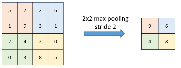
Max pooling layers are similar to convolutions with a 2 x 2 windows and stride of 2, resulting in output feature maps that are half of input width and height.

For instance, before the first MaxPooling2D layers, the feature map is 26 × 26, but the max-pooling operation halves it to 13 × 13. That’s the role of max pooling: to aggressively downsample feature maps, much like strided convolutions.

MNIST Digits Code Example

The following lines of code show that what a basic convnet looks like. It’s a stack of Conv2D and MaxPooling2D layers.

from keras import layers
from keras import models
model = models.Sequential()
model.add(layers.Conv2D(32, (3, 3), activation='relu', input_shape=(28, 28, 1)))
model.add(layers.MaxPooling2D((2, 2)))
model.add(layers.Conv2D(64, (3, 3), activation='relu'))
model.add(layers.MaxPooling2D((2, 2)))
model.add(layers.Conv2D(64, (3, 3), activation='relu'))

Importantly, a convnet takes as input tensors of shape (image_height, image_width, image_channels) (not including the batch dimension). In this case, we’ll configure the convnet to process inputs of size (28, 28, 1), which is the format of MNIST images. It can be done by passing the argument input_shape=(28, 28, 1) to the first layer. Displaying the architecture of the convnet so far by calling model.summary():

Output:

________________________________________________________________
Layer (type) Output Shape Param #
================================================================
conv2d_1 (Conv2D) (None, 26, 26, 32) 320
________________________________________________________________
maxpooling2d_1 (MaxPooling2D) (None, 13, 13, 32) 0
________________________________________________________________
conv2d_2 (Conv2D) (None, 11, 11, 64) 18496
________________________________________________________________
maxpooling2d_2 (MaxPooling2D) (None, 5, 5, 64) 0
________________________________________________________________
conv2d_3 (Conv2D) (None, 3, 3, 64) 36928
================================================================
Total params: 55,744
Trainable params: 55,744
Non-trainable params: 0

The output of every Conv2D and MaxPooling2D layer is a 3D tensor of shape (height, width, channels). The width and height dimensions tend to shrink as going deeper in the network. The number of channels is controlled by the first argument passed to the Conv2D layers (32 or 64).

The next step is to feed the last output tensor (of shape (3, 3, 64)) into a densely connected classifier network: a stack of Dense layers. These classifiers process vectors, which are 1D, whereas the current output is a 3D tensor. First is to flatten the 3D outputs to 1D, and then add a few Dense layers on top.

model.add(layers.Flatten())
model.add(layers.Dense(64, activation='relu'))

model.add(layers.Dense(10, activation='softmax'))

Doing a 10-way classification by using a final layer with 10 outputs and a softmax activation.Displaying the architecture of the convnet so far by calling model.summary():

Layer (type) Output Shape Param #
================================================================
conv2d_1 (Conv2D) (None, 26, 26, 32) 320
________________________________________________________________
maxpooling2d_1 (MaxPooling2D) (None, 13, 13, 32) 0
________________________________________________________________
conv2d_2 (Conv2D) (None, 11, 11, 64) 18496
________________________________________________________________
maxpooling2d_2 (MaxPooling2D) (None, 5, 5, 64) 0
________________________________________________________________
conv2d_3 (Conv2D) (None, 3, 3, 64) 36928
________________________________________________________________
flatten_1 (Flatten) (None, 576) 0
________________________________________________________________
dense_1 (Dense) (None, 64) 36928
________________________________________________________________
dense_2 (Dense) (None, 10) 650
================================================================
Total params: 93,322
Trainable params: 93,322
Non-trainable params: 0

The (3, 3, 64) outputs are flattened into vectors of shape (576,) before going through two Dense layers. Next is to train the CNNs on the MNIST digits.

from keras.datasets import mnist
from keras.utils import to_categorical

(train_images, train_labels), (test_images, test_labels) = mnist.load_data()

train_images = train_images.reshape((60000, 28, 28, 1))
train_images = train_images.astype('float32') / 255
test_images = test_images.reshape((10000, 28, 28, 1))
test_images = test_images.astype('float32') / 255
train_labels = to_categorical(train_labels)
test_labels = to_categorical(test_labels)
model.compile(optimizer='rmsprop', loss='categorical_crossentropy', metrics=['accuracy'])
model.fit(train_images, train_labels, epochs=5, batch_size=64)

Evaluate the model on the test data:

test_loss, test_acc = model.evaluate(test_images, test_labels)
print(test_acc)

Output:

0.99080000000000001

End –Cheng Gu