

Dimensionality Reduction is one of the most popular approaches in unsupervised learning, it provides a way to reduce the complexity of input data. This makes it possible to classify unstructured data by mapping multi-dimensional feature sets to fewer dimensions, such as 3D or 2D.
Common applications of dimensionality reduction include:
PCA is fundamentally a dimensionality reduction algorithm, but it can also be useful as a tool for visualization, noise filtering, feature extraction, engineering, and much more.
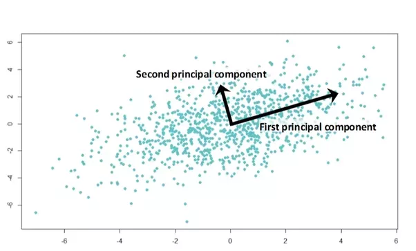
For example, using a 2D dataset, PCA can be used to find a list ofthe principal axes in the data, and using those axes to describe the dataset.
Code Example with Scrit-Learn
import numpy as np
import matplotlib.pyplot as plt
from sklearn.decomposition import PCA

rng = np.random.RandomState(1)
X = np.dot(rng.rand(2, 2), rng.randn(2, 200)).T
pca = PCA(n_components=2)
pca.fit(X)

def draw_vector(v0, v1, ax=None):
    ax = ax or plt.gca()
    arrowprops=dict(arrowstyle='->', linewidth=2, shrinkA=0, shrinkB=0)
    ax.annotate('', v1, v0, arrowprops=arrowprops)

plt.scatter(X[:, 0], X[:, 1], alpha=0.2)
for length, vector in zip(pca.explained_variance_, pca.components_):
    v = vector * 3 * np.sqrt(length)
    draw_vector(pca.mean_, pca.mean_ + v)
plt.axis('equal')
plt.show()
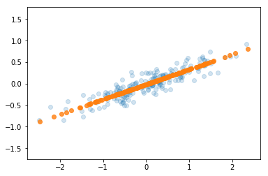
Using PCA for dimensionality reduction involves zeroing out one or more of the smallest principal components, resulting in a lower-dimensional projection of the data that preserves the maximal data variance.
Code Example with Scrit-Learn
import numpy as np
import matplotlib.pyplot as plt
from sklearn.decomposition import PCA

rng = np.random.RandomState(1)
X = np.dot(rng.rand(2, 2), rng.randn(2, 200)).T

pca = PCA(n_components=1)
pca.fit(X)
x_pca = pca.transform(X) # 2D -> 1D
print("Original Shape ",X.shape)
print("Transformed Shape: ",x_pca.shape)

# visualize
X_new = pca.inverse_transform(x_pca) # In order to visualize 1D -> 2D
print(X_new.shape)
plt.scatter(X[:, 0], X[:, 1], alpha=0.2)

plt.scatter(X_new[:, 0], X_new[:, 1], alpha=0.8)
plt.axis('equal')
Output:
End –Cheng Gu