

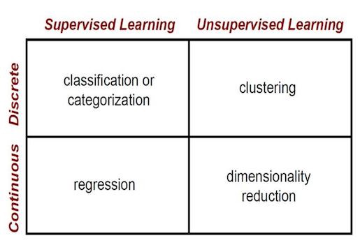
To determine a machine learning whether is supervised learning or unsupervised learning, basicly depends on if the input data(features) has label.Supervised Learning is defined as input data(features) with labels, such as regression and classification. Unsupervised Learning is defined as input data without labels, such as clustering, and dimensional reduction.
“Because we don't give it the answer, it's unsupervised learning”
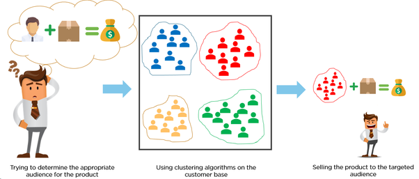
A common case of unsupervised learning is clustering, the process of assigning data to multiple discrete groups. Clustering is a little bit similiar to the classification but it doesn't have label, which means, it doesn't need to care about what a certain category is, the goal is just to gather similar things together. Therefore, clustering algorithm often only needs to know how to calculate the similarity to start working, and it normally doesn't need to use training data for learning.

k-Means is a simple and popular algorithm that searches for a predetermined number of clusters within an unlabeled dataset by following the steps outlined below:
Pseudocode:
randomly choose k examles as initial centroids
while True:
    create k clusters by assigning each example to closest centroid
    compute k new centroids by averaging examples in each cluster
    if centroids don't change:
        break
Code Example with Scrit-Learn
import numpy as np
import matplotlib.pyplot as plt
from sklearn.cluster import KMeans
from sklearn.datasets.samples_generator import make_blobs

# input data, containing 4 blobs
X, y_true = make_blobs(n_samples=500, centers=4, cluster_std=0.40, random_state=0)
plt.scatter(X[:, 0], X[:, 1], s=50)

# initialize and train K-means model with the input data to 4 regions
kmeans = KMeans(n_clusters=4).fit(X)

# predict the results
y_kmeans = kmeans.predict(X)

# assign the predicted results into the color element to visualize
plt.scatter(X[:, 0], X[:, 1], c=y_kmeans, s=50, cmap='viridis')

# plot the center of each region
centers = kmeans.cluster_centers_
plt.scatter(centers[:, 0], centers[:, 1], c='red', s=100, alpha=1.0);
plt.show()
Output:


Meanshift looks very similiar to K-Means, they both move the point closer to the cluster centroids. However, the difference between them is that Meanshift doesn't require to specify the number of clusters, but it is slower than the K-Means in terms of runtime complexity!
Pseudocode:
while not converges:
    for each data point:
        fix a data_range
    calculate the data center in the data_range
    Move the data_range to the new center
Code Example with Scrit-Learn
import numpy as np
import matplotlib.pyplot as plt
from sklearn.cluster import MeanShift, estimate_bandwidth
from sklearn.datasets.samples_generator import make_blobs

# input data, containing 4 blobs
X, y_true = make_blobs(n_samples=500, centers=4, cluster_std=0.40, random_state=0)
plt.scatter(X[:, 0], X[:, 1], s=50)
# Estimate the bandwidth of X
'''
# Bandwidth affects the overall convergence speed and the final number of clusters
# If the bandwidth is small, it might results in too many clusters,
# where as if the value is large, then it will merge distinct clusters.
'''
'''
The quantile parameter impacts how the bandwidth is estimated.
higher value for quantile will increase the estimated bandwidth,
resulting in a lesser number of clusters
'''
bandwidth_X = estimate_bandwidth(X, quantile=0.1,n_samples=len(X))

# Initialize and train the model using the estimated bandwidth
'''
bin_seeding : boolean, optional
If true, initial kernel locations are not locations of all points,
but rather the location of the discretized version of points,
where points are binned onto a grid whose coarseness corresponds to the bandwidth.
Setting this option to True will speed up the algorithm because fewer seeds will be initialized.
'''
model = MeanShift(bandwidth=bandwidth_X,bin_seeding=True).fit(X)
y_meanshit = model.predict(X)
plt.scatter(X[:, 0], X[:, 1], c=y_meanshit, s=50, cmap='viridis')

# Extract the centers of clusters
centers = model.cluster_centers_
print('\nCenters of clusters:\n', cluster_centers)

plt.scatter(centers[:, 0], centers[:, 1], c='red', s=100, alpha=1.0);
plt.show()
Output:
Due to the non-probabilistic nature of k-means and its use of simple distance-from-cluster-center to assign cluster membership leads to poor performance for many real-world situations. As we can see, the mode of clustering by using k-means must be a circle, and it doesn’t have built-in method to calculate oblong or elliptical clusters. Hence, the gaussian mixture model is established. The gaussian mixture model (GMM) attempts to find a mixture of multidimensional gaussian probability distributions to simulate any input data set.
Pseudocode:
choose starting guesses for the location and shape
while not converges:
    # E-step
    for each data point:
        find weights encoding the probability of membership in each cluster
    # M-step
    for each cluster
        update its location, normalization, and shape based on all data points, making use of the weights
Code Example with Scrit-Learn
import numpy as np
import matplotlib.pyplot as plt
from sklearn.mixture import GMM
from sklearn.datasets.samples_generator import make_blobs

# input data, containing 4 blobs
X, y_true = make_blobs(n_samples=500, centers=4, cluster_std=0.40, random_state=0)
plt.scatter(X[:, 0], X[:, 1], s=50)

# initialize gmm and train it
gmm = GMM(n_components=4).fit(X)

#predict result
labels = gmm.predict(X)
plt.scatter(X[:, 0], X[:, 1], c=labels, s=40, cmap='viridis')
Output:

If the data is naturally organized into a number of distinct clusters, then it is easy to visually examine it and draw some inferences. But this is rarely the case in the real world. The data in the real world is huge and messy, so we need a way to quantify the quality of the clustering.
Silhouette is a way to evaluate the clustering quality. The range of the Silhouette Score is between -1 and 1
Formula: $\Large\frac{silhouette score = (p - q)}{ max(p, q)}$
pis themean distanceto the points in thenearestcluster that the data point is not a part ofqis themean intra-cluster distancetoallthe points in itsowncluster.

Code Example with Scrit-Learn
import numpy as np
import matplotlib.pyplot as plt
from sklearn import metrics
from sklearn.cluster import KMeans
from sklearn.datasets.samples_generator import make_blobs

# input data, containing 4 blobs
X, y_true = make_blobs(n_samples=500, centers=4, cluster_std=0.40, random_state=0)

# Initialize variables
scores = []
values = np.arange(2, 10)
print(values)

# Iterate through the defined range
for num_clusters in values:
    # Train the KMeans clustering model
    kmeans = KMeans(init='k-means++', n_clusters=num_clusters, n_init=10)
    kmeans.fit(X)
    score = metrics.silhouette_score(X, kmeans.labels_,
                metric='euclidean', sample_size=len(X))

    print("\nNumber of clusters =", num_clusters)
    print("Silhouette score =", score)

    scores.append(score)

# Plot silhouette scores
plt.bar(values, scores, width=0.7, color='black',
align='center')

# Extract best score and optimal number of clusters
num_clusters = np.argmax(scores) + values[0]
print('\nOptimal number of clusters =', num_clusters)
Output:
Number of clusters = 2
Silhouette score = 0.5983028377054385

Number of clusters = 3
Silhouette score = 0.6735963463903952

Number of clusters = 4
Silhouette score = 0.7900520050938619

Number of clusters = 5
Silhouette score = 0.6829517395665077

Number of clusters = 6
Silhouette score = 0.563136216297564

Number of clusters = 7
Silhouette score = 0.4525060848311459

Number of clusters = 8
Silhouette score = 0.3264185389751767

Number of clusters = 9
Silhouette score = 0.3248083544292323

Optimal number of clusters = 4

End –Cheng Gu