What is Regression?

In contrast to classification, which involves predicting discrete class labels, regression involves predicting continuous quantities.

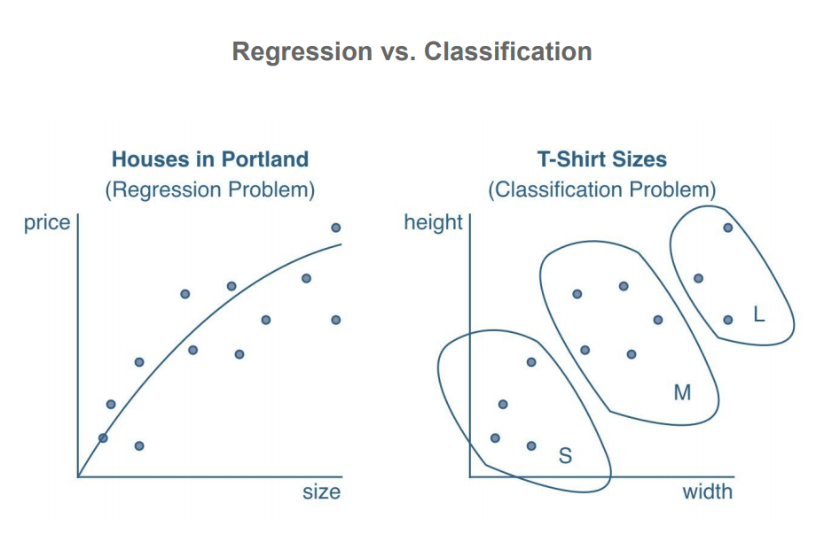
Regression analysis helps in understanding how the value of an output variable changes when we vary some input variables, while keeping other input variables fixed.

It is assumed that the output variables depend on the input variables, so inputs(x) are called independent variables(outcome) and outputs(y) are called dependent variables(preditor).

1. Linear Regression

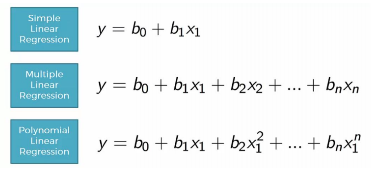
Regression typically involves approximating a mapping function (f) from input variables (x) to a continuous output variable (y). In linear regression, the relationship between input and output can be represented by the line equation:

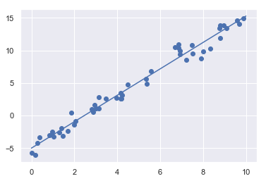
Code Example:

import matplotlib.pyplot as plt
import seaborn as sns; sns.set()
import numpy as np
from sklearn.linear_model import LinearRegression

rng = np.random.RandomState(1)
x = 10 * rng.rand(50)
y = 2 * x - 5 + rng.randn(50)
plt.scatter(x, y); # plot the random points

model = LinearRegression(fit_intercept=True) # get the linear regression model

model.fit(x[:, np.newaxis], y) # train the model

xfit = np.linspace(0, 10, 1000)
yfit = model.predict(xfit[:, np.newaxis])

plt.plot(xfit, yfit); # plot the predicted line

Output:

2. Multiple Linear Regression

The LinearRegression estimator is much more capable than this, however—in addition to simple straight-line fits, it can also handle multidimensional linear models of the form, where there are multiple x values. Geometrically, this is akin to fitting a plane to points in three dimensions, or fitting a hyper-plane to points in higher dimensions.

The multidimensional nature of such regressions makes them more difficult to visualize, but we can see one of these fits in action by building some example data, using NumPy’s matrix multiplication operator:

rng = np.random.RandomState(1)
X = 10 * rng.rand(100, 3)
y = 0.5 + np.dot(X, [1.5, -2., 1.])

model.fit(X, y)
print(model.intercept_)
print(model.coef_)

Output:

0.5
[ 1.5 -2.   1. ]

Here the y data is constructed from three random x values, and the linear regression recovers the coefficients used to construct the data.

In this way, we can use the single LinearRegression estimator to fit lines, planes, or hyperplanes to our data. It still appears that this approach would be limited to strictly linear relationships between variables, but it turns out we can relax this as well.

3. Polynomial basis Functions Regression

When linear regression is not sufficient to map the relationship between input and output, polynomial regression provides a more complex mapping with additional variables and the polynomial function.

Code Example:

import numpy as np
import matplotlib.pyplot as plt
import seaborn as sns; sns.set()
from sklearn.pipeline import make_pipeline
from sklearn.linear_model import LinearRegression
from sklearn.preprocessing import PolynomialFeatures

x = np.array([2, 3, 4])
poly = PolynomialFeatures(3, include_bias=False) # b0+b1x1+b2x1^2+b3x1^3
z=poly.fit_transform(x[:,None]) #Fit to data, then transform it to polynomial features

poly_model = make_pipeline(PolynomialFeatures(7),LinearRegression())

rng = np.random.RandomState(1)
x = 10 * rng.rand(50)
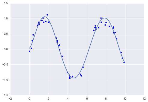
y = np.sin(x) + 0.1 * rng.randn(50)
xfit = np.linspace(0, 10, 1000)
poly_model.fit(x[:, np.newaxis], y) # fit polynomial model
yfit = poly_model.predict(xfit[:, np.newaxis])

plt.scatter(x, y)
plt.plot(xfit, yfit)

Output:

4. Gaussian Basis Functions Regression

Of course, other basis functions are possible. For example, one useful pattern is to fit a model that is not a sum of polynomial bases, but a sum of Gaussian bases. The result might look something like the following figure:

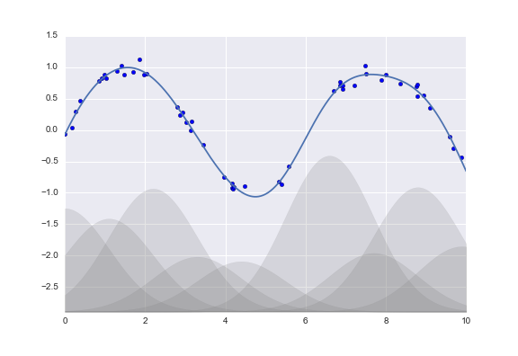
The shaded regions in the plot are the scaled basis functions, and when added together they reproduce the smooth curve through the data.

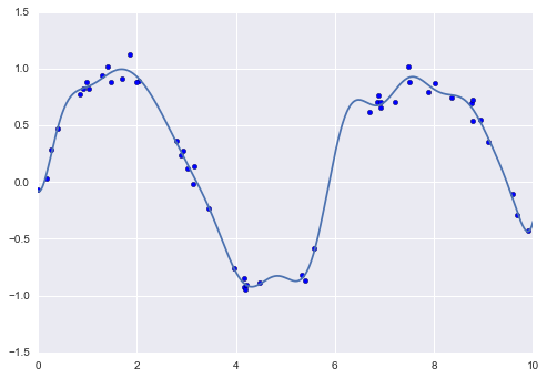
These Gaussian basis functions are not built into Scikit-Learn, but we can write a custom transformer that will create them, as shown here and illustrated in the following figure (Scikit-Learn transformers are implemented as Python classes; reading Scikit-Learn’s source is a good way to see how they can be created):

Code Example:

import numpy as np
import matplotlib.pyplot as plt
import seaborn as sns; sns.set()
from sklearn.pipeline import make_pipeline
from sklearn.linear_model import LinearRegression
from sklearn.base import BaseEstimator, TransformerMixin

class GaussianFeatures(BaseEstimator, TransformerMixin):
    """Uniformly spaced Gaussian features for one-dimensional input"""
    
    def __init__(self, N, width_factor=2.0):
        self.N = N
        self.width_factor = width_factor
    
    @staticmethod
    def _gauss_basis(x, y, width, axis=None):
        arg = (x - y) / width
        return np.exp(-0.5 * np.sum(arg ** 2, axis))
        
    def fit(self, X, y=None):
        # create N centers spread along the data range
        self.centers_ = np.linspace(X.min(), X.max(), self.N)
        self.width_ = self.width_factor * (self.centers_[1] - self.centers_[0])
        return self
        
    def transform(self, X):
        return self._gauss_basis(X[:, :, np.newaxis], self.centers_, self.width_, axis=1)
    
gauss_model = make_pipeline(GaussianFeatures(20),LinearRegression())

rng = np.random.RandomState(1)
x = 10 * rng.rand(50)
y = np.sin(x) + 0.1 * rng.randn(50)
gauss_model.fit(x[:, np.newaxis], y)
xfit = np.linspace(0, 10, 1000)
yfit = gauss_model.predict(xfit[:, np.newaxis])

plt.scatter(x, y)
plt.plot(xfit, yfit)
plt.xlim(0, 10)

Output:

Overfitting vs. Underfitting

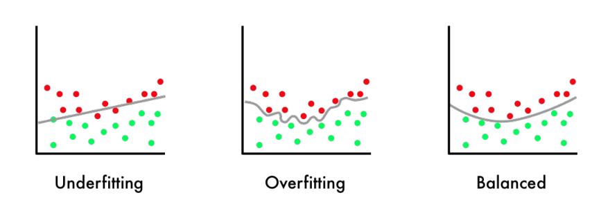
More complex functions, such as Polynomial Regression or Gaussian Rgression, don’t always result in a better model. In contrast to an underfit model that is too simple to describe input data, the model is said to overfit the target when it is too complex for input data. In all, simple but works is better!

End –Cheng Gu